This is a non-state-of-art read through of Stochastic Variance Reduced Gradient (SVRG) [1] method. Gradient descent and stochastic gradient descent (SGD) plays the most important role in optimization of machine learning problems. With large scale datasets, especially in deep learning applications, SGD and its variants maybe the only practical choice. This paper proposes to accelerate the convergence of SGD by reducing the variance of gradient, introduced by random sampling when evaluating gradient. This work has been extended to many other problems, such as non-convex optimization, sparse learning, etc. So this post is just a late bird note.
Gradient Descent and Stochastic Gradient Descent
In machine learning, we usually consider the following optimization problem, $$ \min P(w), \quad P(w) := \frac{1}{n} \sum_{i=1}^n \psi_i(w), $$ where $w$ represents the model parameter and $\psi_i(w)$ is a sequence of loss functions that evaluate the cost of current parameter $w$. Usually, $\psi_i(w)$ depends on training data $(x_i, y_i)$ (supervised learning).
Examples
- square loss: $\psi(w) = (w^T x_i - y_i)^2$
- log loss: $-y_i \ln(\sigma(w^T x_i)) - (1-y_i) \ln(1- \sigma(w^T x_i)) = \ln(1 + \exp(-y_i w^T x_i))$, $\sigma(\cdot)$ is the sigmoid function
Gradient Descent
Gradient descent is derived from the taylor expansion of a function. For smooth $P(w)$, in a small neighborhood of $w_0$, we have $$ P(w) \approx P(w_0) + \langle x - x_0, \nabla f(x_0) \rangle $$
Or along an arbitrary unit direction $d$, we have for small $t > 0$, $$ P(w_0 + td) \approx P(w_0) + t \nabla P(w_0)^T d $$
It turns out that for the negative $d = -\nabla P(w_0)$ is a locally descent direction, that is, for small $t>0$, the following inequality holds, $$ P(w_0 - t \nabla P(w_0)) \approx P(w_0) - t \| \nabla P(w_0)\|_2^2 \leq P(w_0) $$
This leads the standard gradient descent method, $$ w_t = w_{t-1} - \eta_t \nabla P(w_{t-1}) $$
In our problem, we have $\nabla P(w_{t-1}) = \frac{1}{n} \sum_{i=1}^n \nabla \psi_i(w_{t-1})$. I need another post to review the selection of step length $\eta_t$ (aka. learning rate in machine learning), the convergence of gradient descent and recent theoretical results.
Stochastic Gradient Descent
At each step, gradient descent requires evaluations of $n$ derivatives. It is very expensive for large scale problems, which is common in machine leanring. A popular variant is SGD method with the following update rule, $$ w_t = w_{t-1} - \eta_t \nabla \psi_{i_t}(w_{t-1}), $$
where $i_t$ is randomly drawn from $\{1, 2, \ldots, n \}$ at each iteration $t$. We have $\mathbb{E}[\nabla \psi_{i_t}(w_{t-1}) | w_{t-1}] = \nabla P(w_{t-1})$.
Generalized form
The SGD updating rule can be further generalized, $$ w_t = w_{t-1} - \eta_t g_t(w_{t-1}, \xi_t) $$
where $\xi_t$ is a random variable that may depend on $w_{t-1}$ and $g_t(\cdot)$ is an approximate gradient. We only require it is an unbiased estimator, $\nabla P(w_{t-1}) = \mathbb{E}_{\xi_t}[g_t(w_{t-1}, \xi_t)|w_{t-1}]$. For example, the widely used mini-batch version, $$ g_t(w_{t-1}, \xi_t) = \frac{1}{m} \sum_{i=1}^m \nabla \psi_{i_m}(w_{t-1}). $$
Actually, many algorithms use a biased estimator, especially in neural network training. I need another post to reivew the SGD variants and the theoretical results.
Why SVRG
Disadvantages of GD and SGD
| Time Complexity | learning rate | Convergence Rate (Stronly Convex) | |
|---|---|---|---|
| GD | n gradient evaluataion | const. | O(log t) |
| SGD | 1 gradient evaluation | O(1/t) | O(1/t) |
As the stochastic gradient is just a random approximation (by a small batch of samples or even a single example) of the batch gradient, we must be careful when updating along the direction. In order to ensure convergence, the learning rate $\eta_t$ has to decay to zero, due to the variance of random sampling. We generally choose $\eta_t = O(1/t)$. Small learning rate leads to solwer sub-linear convergence rate of $O(1/t)$. We have a trade-off between the computation per iteration and convergence rate.
Fortunately, one can design methods that can reduce the variance of stochastic gradient. This may allow us to use a larger learning rate for SGD.
SVRG algorithm
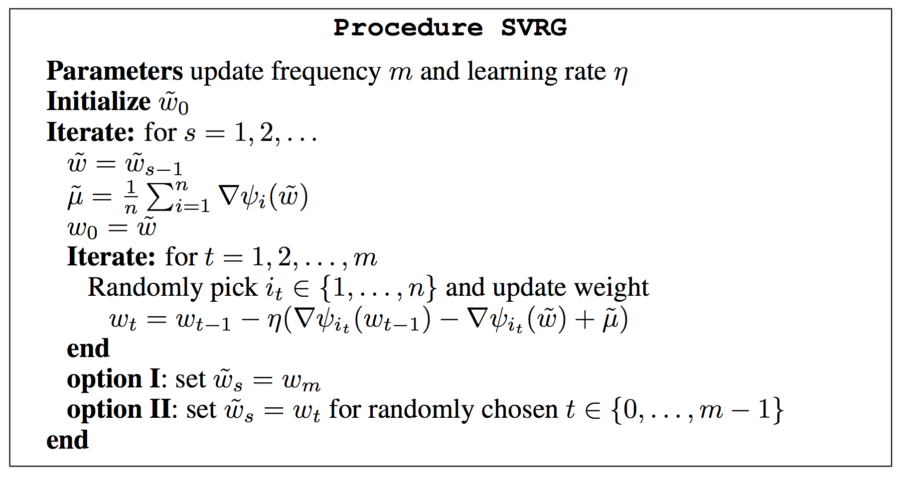
The proposed SVRG algorithm updates by the following rule, $$
w_t = w_{t-1} - \eta_t (\nabla \psi_{i_t}(w_{t-1}) - \nabla \psi_{i_t}(\tilde{w}) + \nabla P(\tilde{w})), $$ where $\tilde{w}$ is a snapshot that is updated every $m$ SGD iterations.
Intuitions
If the snapshot $\tilde{w}$ is close to optima $w^\ast$, $\nabla \psi_i(\tilde{w}) \rightarrow \nabla \psi_i(w^\ast)$,
- Let $\tilde{\mu} := \nabla P(\tilde{w})$, then $\tilde{\mu} - \nabla P(w_{t-1}) \approx \nabla \psi_i(\tilde{w}) - \nabla \psi_i(w_{t-1})$. Intuitively, this updating rule cancel the randomness induced by random sampling $i$;
- $\tilde{\mu} \rightarrow 0$ when $\tilde{w} \rightarrow w^\ast$. $\nabla \psi_i(w_{t-1}) - \nabla \psi_i(\tilde{w}) + \tilde{\mu} \rightarrow \nabla \psi_i(w_{t-1}) - \nabla \psi_i(w^\ast) \rightarrow 0$. The infinite small gradient allows to use constant learning rate. However, for SGD, $\nabla \psi_i(w_{t-1})$ may not converge to 0.
Algorithm

Theorem
Suppose $\gamma$-smooth $\psi_i$ and $L$-strongly convex $P(w)$. Let $w^\ast = \arg \min_w P(w)$. We have geometric convergence in expectation for SVRG: $$\mathbb{E} P(\tilde{w}_s) - \mathbb{E} P(w^\ast) \leq \alpha^s (P(\tilde{w}_0) - P(w^\ast))$$ given $m$ is sufficiently large, s.t., $$\alpha = \frac{1}{\gamma \eta m(1-2L\eta)} + \frac{2L \eta}{1-2L \eta} < 1$$
Actually, $m$ is of the same order of $n$ in the paper. Thus it might be more precise to say the following convergence rate, $$ \mathbb{E} P(\tilde{w}_s) - \mathbb{E} P(w^\ast) \leq \alpha^{t/n} (P(\tilde{w}_0) - P(w^\ast))$$
Summary
- Randomness of SGD induces variance of gradient, which leads to decay learning rate and sub-linear convergence rate
- Reducing the variance of stochastic gradient allows to use constant learning rate and obtains linear convergence in expectation
- We donnot need to save the historical gradient $\nabla \psi_{i_1}(w_0), \nabla \psi_{i_2}(w_1), \ldots$ in SVRG. However, the number of gradient evaluation per iteration increases
- SVRG may be applied to non-strongly convex problem, leading a $O(1/T)$ convergence rate (standard SGD $O(1/\sqrt{T})$)
- SVRG can also be used to non-convex optimization problem, such as neural networks training
Johnson, Rie, and Tong Zhang. “Accelerating stochastic gradient descent using predictive variance reduction.” In Advances in Neural Information Processing Systems, pp. 315-323. 2013. ↩